

Servo dynamics
Measured on 2026-10-04 from the Raspberry Pi 5 (direct bus, allocation-free loop,
334 Hz). Recordings: tools/python/recordings/sysid/.
Method
Section titled “Method”scripts/sysid.jl moves one joint at a time while the others hold zero. A
chirp sweeps 0.2 → 5 Hz (logarithmic). Its amplitude is limited so that the
speed stays below --vmax and the acceleration below --amax.
tools/python/analyze_sysid.py estimates the frequency response from the commanded
to the measured position, and fits a second-order model.
julia --project=. scripts/sysid.jl 1 chirp --amp=10 --vmax=120 --amax=300python3 tools/python/analyze_sysid.py tools/python/recordings/sysid/<file>.csv --plot out.pngThe servos have an acceleration limit
Section titled “The servos have an acceleration limit”A 10° chirp on J1 follows well up to ~1 Hz, and then the amplitude falls quickly. With 3° the knee moves to ~2 Hz. A linear system does not do this. The knee is where the sine needs more than ~440°/s²: the J1–J3 servos limit their acceleration.
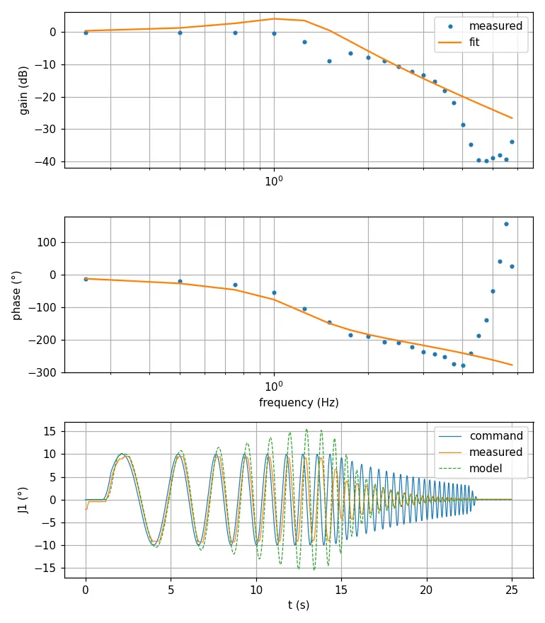
- The limit is the factory register 85 (maximum acceleration) × 100 steps/s²: 50 on J1–J3 (≈ 440°/s²) and 250 on J4–J6 (≈ 2200°/s²).
- Register 41 (acceleration) is clamped to register 85. After a write of 254 it read 50 on J1–J3 and 250 on J4–J6. A run with 254 was the same as a run with 0.
- So at the default settings, J1–J3 cannot accelerate faster than ~440°/s². Plans must stay below this, or the servo falls behind. The old lag numbers (~120 ms on J1–J3) partly came from this saturation.
Register 85 is a factory setting. It is not changed: a higher limit could be possible, but it can be there to protect the gears.
Second-order model inside the limit
Section titled “Second-order model inside the limit”With the acceleration limited (300°/s² on J1–J3, 1500°/s² on J4–J6), each joint
follows like a linear second-order system: q/goal = ωn² / (s² + 2ζωn s + ωn²).
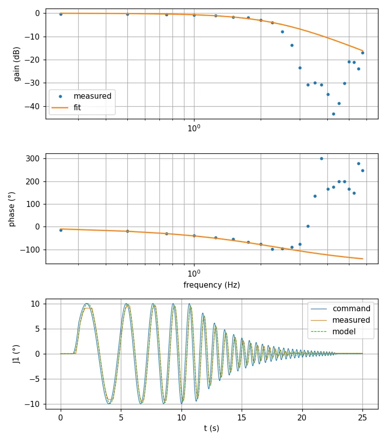
| Joint | ωn (rad/s) | ζ | Equivalent delay at low frequency | Model RMS | Pure-delay RMS |
|---|---|---|---|---|---|
| J1 | 14.8 | 0.82 | ~108 ms | 0.22° | 0.39° |
| J2 | 14.7 | 0.75 | ~105 ms | 0.32° | 0.35° |
| J3 | 14.2 | 0.78 | ~110 ms | 0.24° | 0.37° |
| J4 | 34.4 | 0.65 | ~40–50 ms | 0.37° | 0.35° |
| J5 | 52.4 | 0.77 | ~25–40 ms | 0.41° | 0.41° |
| J6 | 54.9 | 0.83 | ~25–40 ms | 0.39° | 0.39° |
The values are in src/servo_model.jl (SERVO_WN, SERVO_ZETA, SERVO_AMAX).
J1–J3 are the same servo type (model 0x0809) and have the same dynamics.
Model feedforward
Section titled “Model feedforward”MyCobot.model_feedforward(t, q) inverts the model: u = q + (2ζ/ωn) q̇ + q̈/ωn².
The derivatives are smoothed (60 ms zero-phase average), because the plans are made
of segments with acceleration jumps. Use it with
scripts/play_plan.jl <plan> --ff=model.
On the circle (2026-10-04, Raspberry Pi):
| Commands | Flange error RMS | Max |
|---|---|---|
| Lag compensation (time shift) | 5.1 mm | 12.2 mm |
| Model feedforward | 5.1 mm | 11.8 mm |
Recordings: tools/python/recordings/20261004-144010_circle_lagcomp_jl.csv and
20261004-144047_circle_modelff_jl.csv.
The model feedforward removes the modelled part of the error completely (the model’s prediction equals the plan to 0.01°). The remaining error is not in the model: 0.3–0.4° on J1, J4, J5 and 0.9–1.1° on J2 and J3, the joints that carry the arm. It correlates with the load (r = 0.87 on J2 and J3) and with the pose: gravity and friction with almost no integral action in the servos (I = 0 on J1–J2, 1 on J3–J6).
Servo gains (PID) and the IMU
Section titled “Servo gains (PID) and the IMU”The servos run a position loop with gains P, D, I (registers 21, 22, 23). With the custom firmware all six use their stored values 32/8/0: no integral action. (The stock firmware writes 10/0/1 to J3–J6 at power-up; see Servos.) Changes last until the next power cycle.
Steps at a loaded pose (J2 and J3)
Section titled “Steps at a loaded pose (J2 and J3)”scripts/sysid.jl 2 steps --amp=5 --T=24 --base=0,-30,-60,0,0,0 --pid=P,D,I:
±5° steps around a pose where gravity loads J2 and J3, 3 s holds.
| Gains (P/D/I) | J2 steady error mean / max | J3 steady error mean / max |
|---|---|---|
| 32/8/0 (default) | 1.34° / 2.17° | 0.84° / 1.61° |
| 64/16/0 | 0.69° / 0.94° | — |
| 64/16/4 | 0.41° / 0.79° | 0.36° / 0.62° |
| 96/24/4 | 0.42° / 0.62° | 0.34° / 0.46° |
With P only, the joint settles short of the target under load (droop ∝ 1/P). The servo encoders show no extra jitter at higher gains.
The circle on the ATOM, with the IMU
Section titled “The circle on the ATOM, with the IMU”The servo encoders do not show everything. The IMU at the end effector does:
high P gains make the arm vibrate during motion, although the joints look quiet.
Circle, lag compensation, onboard at 500 Hz; gains on J1–J3 (J4–J6 at 32/8/0);
vibration = IMU signal above ~2.5 Hz (tools/python/imu_vibration.py):
| Gains J1–J3 (P/D/I) | Flange error RMS / max | Acceleration RMS | Rotation rate RMS |
|---|---|---|---|
| 32/8/0 (default, 4 runs) | 5.0–5.3 mm / 11.9–12.9 mm | 151–158 mg | 9.7–10.3°/s |
| 96/24/4 | 4.8 / 7.7 mm | 624 mg | 49°/s |
| 96/8/4 | 4.8 / 8.0 mm | 611 mg | 48°/s |
| 64/8/4 | 3.8 / 6.7 mm | 391 mg | 31°/s |
| 48/4/4 | 3.0 / 6.5 mm | 244 mg | 20°/s |
| 32/8/4 | 2.9 / 9.5 mm | 148 mg | 9.9°/s |
| 32/4/16 (3 runs) | 2.4–2.7 / 6.7–8.2 mm | 162–169 mg | 11°/s |
| 32/4/32 | 3.0 / 8.0 mm | 169 mg | 12°/s |
| 32/4/64 | 4.5 / 11.2 mm | 149 mg | 9.5°/s |
- P sets the vibration: 32 → 155 mg, 48 → 244 mg, 64 → ~400 mg, 96 → ~610 mg. D has little effect.
- I gives the precision without the vibration. I = 16 on J1–J3 halves the error (5.3 → 2.6 mm). I = 64 is worse again (overshoot). I on J4–J6 did not help.
- These are now our default gains (
MyCobot.GAINS). The controller firmware v3 writes them at every power-up; see Position-loop gains. - ILC on top of the tuned gains: 2.6 → 1.4 mm after one iteration, then 1.5 and
1.8 mm. It does not converge further with the ILC settings that were tuned for
the default gains (they reached 1.0 mm). The lead time (
DEFAULT_LAG) probably needs an update for the new gains.
What did not work
Section titled “What did not work”A static error map (gravity terms of the pose, friction, inertia), fitted on an
excitation trajectory, reduced the error on a second excitation run (J2 1.01° →
0.56°) but made the circle worse on J2 and J6. The circle uses poses outside the
excitation data (J3 ≈ −103°, J4 up to 120°). A gravity model must be calibrated over
the whole workspace before it can be used.
Recordings: tools/python/recordings/20261004-1444*_excitation_*_modelff_jl.csv.
- Calibrate the steady-state error against gravity over a grid of poses.
- Measure the lag with the tuned gains, then repeat ILC with it.
- For repeated motions, ILC already removes most of the error (0.8 mm).