Open the live demo
Runs in your browser — nothing to install.
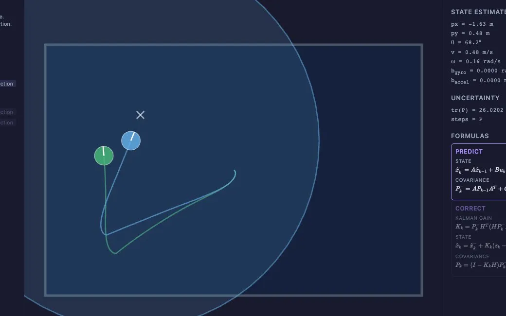
An interactive introduction to robot localization, using a robot vacuum as the example. It is built as a path: each stage adds one idea on top of the last, and you toggle sensors on and off to see why it matters.
- Dead reckoning — wheel encoders alone. Errors accumulate without correction.
- Kalman filter — add an IMU. The filter fuses the encoder prediction with IMU measurements to correct drift.
- Localization — add LiDAR and a known map for absolute position. Uncertainty drops dramatically.
- SLAM — build the map while navigating (coming soon).
The robot is driven by a closed-loop planner that uses the filter’s own estimate — so a poorly tuned filter visibly degrades navigation, just as it would on real hardware.
What’s modelled
- Ground truth — unicycle kinematics for a differential-drive robot.
- Wheel encoders — noisy v and ω, with wheel-diameter mismatch and slip (the prediction input).
- IMU (MPU-6050) — raw gyro and accelerometer with drifting biases.
- LiDAR — presets for RPLiDAR A1/A2, Hokuyo URG-04LX, and SICK TIM561, with realistic beam counts, range noise, and update rates.
- 7-state EKF —
[px, py, θ, v, ω, b_a, b_g]with online bias estimation.
The control loop runs at 200 Hz, decoupled from the ~60 Hz display, and each sensor fires at its own rate. The matrix maths is hand-rolled and kept explicit for educational clarity.